Bonate (2011): Pharmacokinetic-Pharmacodynamic Modeling and Simulations

Here, we replicate some of the examples described in Bonate (2011). I recommend following along with the 2nd edition of the book. The purpose of this notebook is to illustrate the versatility of delicatessen by illustrating its application for pharmacokinetic modeling. This can easily be done by using the built-in estimating equations, as will be shown.

Bonate PL. (2011). Pharmacokinetic-Pharmacodynamic Modeling and Simulations. 2nd Edition. Springer, New York, NY.

Setup

import numpy as np
import scipy as sp
import pandas as pd
import statsmodels.api as sm
import statsmodels.formula.api as smf
import matplotlib.pyplot as plt

import delicatessen as deli
from delicatessen import MEstimator
from delicatessen.estimating_equations import ee_emax, ee_glm
from delicatessen.utilities import aggregate_efuncs

np.random.seed(80950841)

print("NumPy version:       ", np.__version__)
print("SciPy version:       ", sp.__version__)
print("Pandas version:      ", pd.__version__)
print("Delicatessen version:", deli.__version__)

NumPy version:        2.3.5
SciPy version:        1.16.3
Pandas version:       2.3.3
Delicatessen version: 4.1

Chapter 4: Variance Models, Weighting, and Transformations

The first example comes from Chapter 4. Data comes from Table 9 (pg 153) from a study by Byers et al. (1989) on XomaZyme-791 dose on percent change in albumin concentration among 17 patients. Note that this number of patients may be below what is considered sufficient for inference with the sandwich.

The E-max model is described by

\[R_i = E_0 + (E_{m} - E_0) \frac{D_i}{ED_{50} + D_i}\]

where \(D\) is the dose, \(R\) is the response, \(E_0\) is the response at a dose of zero, \(E_m\) is the maximum response, and \(ED_{50}\) is the halfway maximal dose. Here, \(E_0 = 0\) so the E-max model reduces to

\[R_i = E_{m} \frac{D_i}{ED_{50} + D_i}\]

This is the model we will consider.

The corresponding data is presented below

d = [5, 5, 13, 11, 14.5, 6.8, 42.5, 37.5, 25, 38, 40, 26.5, 27.7, 27.4, 45, 61.4, 52.8]
r = [-12, -13, -28, -24, -45, -18, -26, -40, -45, -26, -29, -26, -22, -28, -36, -27, -48]

In the book, a two parameter E-max model is used. The first parameter is maximum response and the second is the 50% effective dose. The minimum dose will be set as zero (i.e., not estimated) since there is no data on a dose of zero.

Here, we will apply the same linear model described in the book (i.e., prior to the Box-Cox transformation). This can be done using the ee_emax built-in estimating equation. But before that, we will plot the dose-response data. This is an important step, as it will help us decided on starting values for the root-finding procedure

plt.plot(d, r, 'o', color='gray')
plt.xlabel("Dose")
plt.ylim([-50, 0])
plt.ylabel("Response")
plt.xlim([0, 70])
plt.tight_layout()

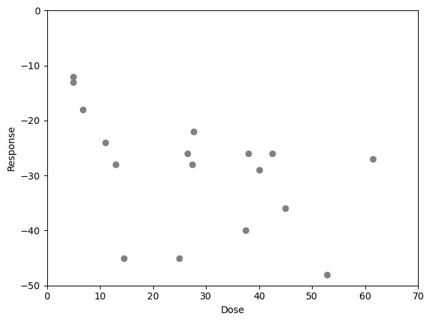
Given this dose-response data, it appears that the dose-response begins to asymptote at some point beyond a dose of 10. Therefore, we should select a starting value of \(ED_{50}\) below 10. Further, a maximum response value between -30 and -50 seems reasonable, so we will select -40 as the max effect starting value.

def psi(theta):
    lower = 0
    vals = [0., ] + list(theta)
    return ee_emax(theta=vals, dose=d, response=r)[1:, :]

estr = MEstimator(psi, init=[-40, 5])
estr.estimate()

# Setting up a Table for the results
results = pd.DataFrame()
results['Params'] = ["E-max", "ED50"]
results = results.set_index('Params')
results['Est'] = estr.theta
results['SE'] = np.diag(estr.variance) ** 0.5
ci = estr.confidence_intervals()
results['LCL'] = ci[:, 0]
results['UCL'] = ci[:, 1]
results.round(1)

	Est	SE	LCL	UCL
Params
E-max	-38.6	4.1	-46.7	-30.5
ED50	6.2	2.4	1.5	10.9

These results are close to what is reported in the book (note that a different variance estimator is used).

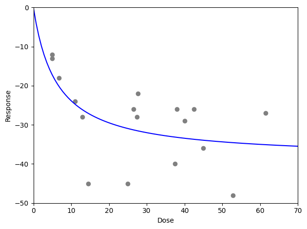
We can also use these parameters to generate a plot.

x = np.linspace(0, 70, 100)
y = estr.theta[0] * x / (estr.theta[1] + x)

plt.plot(d, r, 'o', color='gray')
plt.plot(x, y, '-', color='blue')
plt.xlabel("Dose")
plt.ylim([-50, 0])
plt.ylabel("Response")
plt.xlim([0, 70])
plt.tight_layout()

While not discussed in the chapter, one might be concern about outlying response values. Particularly, there are some large responses at low doses. These few response values might be overly influential on the overall E-max parameter estimates. To go beyond the book, we can consider the use of outlier-robust estimating functions. These apply an additional constraint that limits the maximum influence an observation can have to the estimating function. The following code uses the Huber function to limit the influence.

def psi_robust(theta):
    lower = 0.
    vals = [lower, ] + list(theta)
    return ee_emax(theta=vals, dose=d, response=r, robust='huber', k=5.)[1:, :]


estr = MEstimator(psi_robust, init=[-40, 5])
estr.estimate(solver='lm')

results = pd.DataFrame()
results['Params'] = ["E-max", "ED50"]
results = results.set_index('Params')
results['Est'] = estr.theta
results['SE'] = np.diag(estr.variance) ** 0.5
ci = estr.confidence_intervals()
results['LCL'] = ci[:, 0]
results['UCL'] = ci[:, 1]
results.round(1)

	Est	SE	LCL	UCL
Params
E-max	-35.5	4.2	-43.7	-27.4
ED50	6.3	2.1	2.3	10.3

y2 = estr.theta[0] * x / (estr.theta[1] + x)

plt.plot(d, r, 'o', color='gray')
plt.plot(x, y, '-', color='blue')
plt.plot(x, y2, '-', color='green')
plt.xlabel("Dose")
plt.ylim([-50, 0])
plt.ylabel("Response")
plt.xlim([0, 70])
plt.tight_layout()

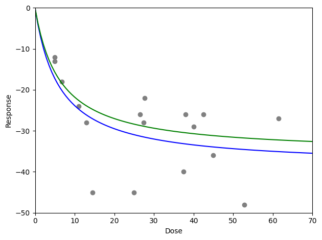
Here, we observe a minor change in the estimated coefficients. In the plot, we can see that the dose-response curve estimated using the outlier-robust approach (green) did not drop as low as the non-robust method (blue). This is expected given the apparent outliers around doses of 15, 25, and 52.

Chapter 9: Nonlinear Mixed Effects Models: Case Studies

This chapter presents some case studies of nonlinear mixed effects models. Here, we will review some of the case studies but modify them to use estimating equations instead.

Pharmacodynamic Modeling of Acetylcholinesterase Inhibition

Data comes from Cutler et al. 1995 and is provided in Table 1 of this chapter (pg 360). Data comes from 12 participants with Zifrosilone dose on inhibition of acetylcholinesterase. Here, multiple measurements were obtained from the same participants over different timings. Here, we will explore the use of E-max models again but with some caveats. First, we load the data set

d = pd.read_csv("data/cutler1995_pd.csv")

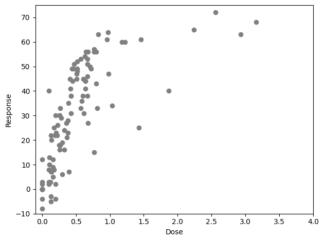
In this data, participants have multiple measures over time. We can easily observe this by plotting our data (which has many more points that 12)

plt.plot(d['zifro'], d['acetyl'], 'o', color='gray')
plt.xlabel("Dose")
plt.ylim([-10, 75])
plt.ylabel("Response")
plt.xlim([-0.1, 4])
plt.tight_layout()

While we will ignore the time-since-dose in this analysis, we should not ignore the fact that a single unit contributes multiple times to estimation. Our variance needs to account for this. Let’s first ignore this aspect and treat all the observations as if they were independent

def psi(theta):
    return ee_emax(theta=theta, dose=d['zifro'], response=d['acetyl'])

estr = MEstimator(psi, init=[0, 60, 0.5])
estr.estimate()

results = pd.DataFrame()
results['Params'] = ["Zero-Dose", "E-max", "ED50"]
results = results.set_index('Params')
results['Est'] = estr.theta
results['SE'] = np.diag(estr.variance) ** 0.5
ci = estr.confidence_intervals()
results['LCL'] = ci[:, 0]
results['UCL'] = ci[:, 1]
results.round(1)

	Est	SE	LCL	UCL
Params
Zero-Dose	-2.3	1.3	-4.9	0.3
E-max	84.5	6.6	71.4	97.5
ED50	0.6	0.1	0.4	0.8

To compare, let’s modify the estimating functions. Here, we will use the aggregate_efuncs to collapse the contributions by unique subject IDs. The dimension of this new estimating functions will be 3-by-12, to reflect the fact that there are only 12 independent observations. The following code applies this process

def psi_c(theta):
    ef_emax_i = ee_emax(theta=theta, dose=d['zifro'], response=d['acetyl'])
    return aggregate_efuncs(ef_emax_i, group=d['subject'])

estr = MEstimator(psi_c, init=[0, 60, 0.5])
estr.estimate()

results = pd.DataFrame()
results['Params'] = ["Zero-Dose", "E-max", "ED50"]
results = results.set_index('Params')
results['Est'] = estr.theta
results['SE'] = np.diag(estr.variance) ** 0.5
ci = estr.confidence_intervals()
results['LCL'] = ci[:, 0]
results['UCL'] = ci[:, 1]
results.round(1)

	Est	SE	LCL	UCL
Params
Zero-Dose	-2.3	1.6	-5.3	0.8
E-max	84.5	7.4	70.0	99.0
ED50	0.6	0.1	0.4	0.7

As seen here, the point estimates are similar but the variance changes.

However, 12 observations is still relatively few so we can further apply a finite-sample correction using the finite_correction optional argument as shown in the following code

estr = MEstimator(psi_c, init=[0, 60, 0.5], finite_correction='HC1')
estr.estimate()

results = pd.DataFrame()
results['Params'] = ["Zero-Dose", "E-max", "ED50"]
results = results.set_index('Params')
results['Est'] = estr.theta
results['SE'] = np.diag(estr.variance) ** 0.5
ci = estr.confidence_intervals()
results['LCL'] = ci[:, 0]
results['UCL'] = ci[:, 1]
results.round(1)

	Est	SE	LCL	UCL
Params
Zero-Dose	-2.3	1.8	-6.3	1.8
E-max	84.5	8.5	65.1	103.8
ED50	0.6	0.1	0.4	0.8

Here, we see the variance increase a bit further (due to the additional correction). This concludes the case study showing how to account for non-independent observations and small sample sizes.

Chapter 11: Generalized Linear Models and Its Extensions

Adverse Events Case Study

The first example from Chapter 11 is the Case Study: Assessing the Relationship Between Drug Concentrations and Adverse Events Using Logistic Regression. Data comes from Table 2 of the book. In the book, a variety of different models for different adverse events are considered. Here, we only consider nausea (and vomiting) by AUC. For the one observations with a missing AUC value, they are dropped from the data set (same as the book). For ease of examining the coefficients, we will also divide the AUC value by 1000. This means the coefficients for AUC are rescaled from those reported in the book.

First, we load the data set and transform the coefficients and add an intercept column to the data set

d = pd.read_csv("data/bonate.csv").dropna()
d['intercept'] = 1   # Adding intercept to data
d['auc'] /= 1000     # Rescaling AUC
d['c_max'] /= 1000   # Rescaling C_max
d.info()

<class 'pandas.core.frame.DataFrame'>
Index: 42 entries, 0 to 42
Data columns (total 12 columns):
 #   Column     Non-Null Count  Dtype
---  ------     --------------  -----
 0   id         42 non-null     int64
 1   c_max      42 non-null     float64
 2   auc        42 non-null     float64
 3   age        42 non-null     int64
 4   sex        42 non-null     int64
 5   ps         42 non-null     int64
 6   myalgia    42 non-null     int64
 7   phlebitis  42 non-null     int64
 8   asthenia   42 non-null     int64
 9   diarrhea   42 non-null     int64
 10  nausea     42 non-null     int64
 11  intercept  42 non-null     int64
dtypes: float64(2), int64(10)
memory usage: 4.3 KB

table = pd.DataFrame(columns=["Model", "Intercept", "AUC", "Sex", "Age", "PS"])

To begin, we will fit a null (intercept-only) logistic regression model. This is easily done by using the built-in ee_glm estimating equation. For the logistic model, we specify a binomial distribution with the logit link. Below is code to setup the estimating equation and then estimate the parameters using MEstimator

def psi(theta):
    # Estimating equation for null model
    return ee_glm(theta=theta,
                  y=d['nausea'],
                  X=d[['intercept', ]],
                  distribution='binomial',
                  link='logit')


# Estimate the parameters of the logit model
estr_null = MEstimator(psi, init=[0., ])
estr_null.estimate()

# Adding results to the output table
table.loc[len(table)] = ["Null", estr_null.theta[0], ] + [np.nan, ]*4

Next we fit a logistic regression model that includes linear terms for all the independent variables in the data set. This is easily done by modifying the previous design matrix (i.e., X). Below is code to fit the full model

def psi(theta):
    # Estimating equation for full model
    return ee_glm(theta=theta,
                  y=d['nausea'],
                  X=d[['intercept', 'auc', 'sex', 'age', 'ps']],
                  distribution='binomial',
                  link='logit')


# Estimate the parameters of the logit model
estr_full = MEstimator(psi, init=[0., ]*5)
estr_full.estimate()

# Adding results to the output table
table.loc[len(table)] = ["Full", ] + list(estr_full.theta)

In the book, Bonate performs some variable selection. In general, we would not recommend use of backwards-selection procedures (like those done in the book). Such procedures complicate inference (P-values and confidence intervals after these procedures are no longer valid). For comparison purposes, we estimate the reduced model reported in the book. Again, this is easily done by modifying the X argument for ee_glm

def psi(theta):
    # Estimating equation for reduced model
    return ee_glm(theta=theta,
                  y=d['nausea'],
                  X=d[['intercept', 'auc', 'sex']],
                  distribution='binomial',
                  link='logit')


# Estimate the parameters of the logit model
estr_redu = MEstimator(psi, init=[0., ]*3)
estr_redu.estimate()

# Adding results to the output table
table.loc[len(table)] = ["Reduced", ] + list(estr_redu.theta) + [np.nan, ]*2

Finally, two alternative models are considered: a probit regression model and a complimentary log-log model. Again, these models are easily implemented using ee_glm. For the probit model, we set the link equal to probit

def psi(theta):
    # Estimating equation for reduced probit model
    return ee_glm(theta=theta,
                  y=d['nausea'],
                  X=d[['intercept', 'auc', 'sex']],
                  distribution='binomial',
                  link='probit')


# Estimate the parameters of the probit model
estr_prob = MEstimator(psi, init=[0., ]*3)
estr_prob.estimate()

# Adding results to the output table
table.loc[len(table)] = ["Probit", ] + list(estr_prob.theta) + [np.nan, ]*2

Similarly, the complimentary log-log model only requires setting the link to cloglog

def psi(theta):
    # Estimating equation for reduced C-log-log model
    return ee_glm(theta=theta,
                  y=d['nausea'],
                  X=d[['intercept', 'auc', 'sex']],
                  distribution='binomial',
                  link='cloglog')


# Estimate the parameters of the cloglog model
estr_clog = MEstimator(psi, init=[0., ]*3)
estr_clog.estimate()

# Adding results to the output table
table.loc[len(table)] = ["CLogLog", ] + list(estr_clog.theta) + [np.nan, ]*2

Now we can view the results across the different models

table.set_index("Model")

	Intercept	AUC	Sex	Age	PS
Model
Null	-0.587787	NaN	NaN	NaN	NaN
Full	-5.602899	0.289785	1.730299	0.049538	0.220545
Reduced	-2.663522	0.303502	1.772238	NaN	NaN
Probit	-1.629729	0.184030	1.080253	NaN	NaN
CLogLog	-2.233720	0.193108	1.212290	NaN	NaN

These point estimates match those reported in Tables 3 and 4 on pages 469 and 470 in the book (note the null model differs slightly, since we dropped the one observation with the missing AUC value to fit this model, but the book does not). These results highlight how delicatessen allows one to easily fit a variety of different models.

This is the end of the current replication.