Built-in Estimating Equations
Here, we provide an overview of some of the built-in estimating equations with delicatessen. This documentation is
split into several sections based on topic areas.
All built-in estimating equations need to be ‘wrapped’ inside an outer function. Below is a generic example of an outer
function, where psi is the wrapper function and ee is the generic estimating equation example (ee is not a
valid built-in estimating equation).
def psi(theta):
    return ee(theta=theta, data=data)
Here, ee takes two inputs theta and data. theta is the general theta vector that is present
in all stacked estimating equations expected by delicatessen. data is an argument that takes an input source
of data. The data provided should be in the local scope of the .py file this function lives in.
After wrapped in an outer function, the function can be passed to MEstimator. See the examples below for further
details and examples.
To replicate the following examples, please load the following libraries as shown
import numpy as np
import pandas as pd
import matplotlib.pyplot as plt
from delicatessen import MEstimator
Basic Equations
Some basic estimating equations are provided.
Mean
The most basic available estimating equation is for the mean: ee_mean. To illustrate, consider we wanted to
estimated the mean for the following data
obs_vals = [1, 2, 1, 4, 1, 4, 2, 4, 2, 3]
To use ee_mean with MEstimator, this function will be wrapped in an outer function. Below is an illustration of
this wrapper function
from delicatessen.estimating_equations import ee_mean

def psi(theta):
    return ee_mean(theta=theta, y=obs_vals)
Note that obs_vals must be available in the scope of the defined function.
After creating the wrapper function, the corresponding M-Estimator can be called like the following
from delicatessen import MEstimator

estr = MEstimator(stacked_equations=psi, init=[0, ])
estr.estimate()

print(estr.theta)   # [2.4, ])
Since ee_mean consists of a single parameter, only a single init value is provided.
Robust Mean
Sometimes extreme observations, termed outliers, occur. The mean is generally sensitive to these outliers. A common approach to handling outliers is to exclude them. However, exclusion ignores all information contributed by outliers, and should only be done when outliers are a result of experimental error. Robust statistics have been proposed as middle ground, whereby outliers contribute to estimation but their overall influence is constrained.
obs_vals = [1, -10, 2, 1, 4, 1, 4, 2, 4, 2, 3, 12]
Instead, the robust mean can be used instead. The robust mean estimating equation is available in ee_mean_robust,
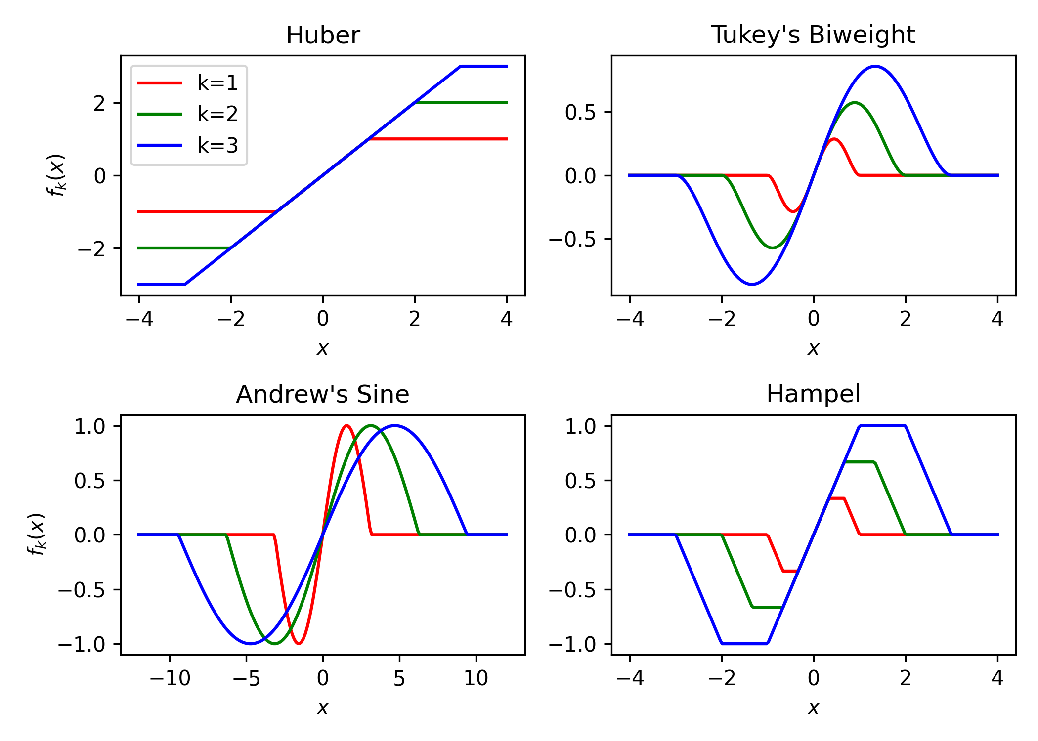
with several different options for the loss function. The following is a plot showcasing the influence functions for
the available robust loss functions.
from delicatessen import MEstimator
from delicatessen.estimating_equations import ee_mean_robust

def psi(theta):
    return ee_mean_robust(theta=theta, y=obs_vals, loss='huber', k=6)

estr = MEstimator(stacked_equations=psi, init=[0, ])
estr.estimate()

print(estr.theta)
Mean and Variance
A stacked estimating equation, where the first value is the mean and the second is the variance, is also provided. Returning to the previous data,
obs_vals = [1, 2, 1, 4, 1, 4, 2, 4, 2, 3]
The mean-variance estimating equation can be implemented as follows
from delicatessen.estimating_equations import ee_mean_variance

def psi(theta):
    return ee_mean_variance(theta=theta, y=obs_vals)

estr = MEstimator(stacked_equations=psi, init=[0, 1, ])
estr.estimate()

print(estr.theta)  # [2.4, 1.44]
Note init here takes two values because there are two parameters. The first value of theta is the mean and
the second is the variance. Now, the variance output provides a 2-by-2 covariance matrix. The leading diagonal of that
matrix are the variances (where the first is the estimated variance of the mean and the second is the estimated
variance of the variance).
Regression
Several common regression models are provided as built-in estimating equations.
Linear Regression
The estimating equations for linear regression predict a continuous outcome as a function of provided covariates.
To demonstrate application, consider the following simulated data set
import numpy as np
import pandas as pd

n = 500
data = pd.DataFrame()
data['X'] = np.random.normal(size=n)
data['Z'] = np.random.normal(size=n)
data['Y1'] = 0.5 + 2*data['X'] - 1*data['Z'] + np.random.normal(loc=0, size=n)
data['Y2'] = np.random.binomial(n=1, p=logistic.cdf(0.5 + 2*data['X'] - 1*data['Z']), size=n)
data['Y3'] = data['Y3'] = np.random.poisson(lam=np.exp(0.5 + 2*data['X'] - 1*data['Z']), size=n)
data['C'] = 1
In this case, X and Z are the independent variables and Y is the dependent variable. Here the column C
is created to be the intercept column, since the intercept needs to be manually provided (this may be different from
other formula-based packages that automatically add the intercept to the regression).
For this data, we can now create the wrapper function for the ee_regression estimating equations
from delicatessen.estimating_equations import ee_regression

def psi(theta):
    return ee_regression(theta=theta,
                         X=data[['C', 'X', 'Z']],
                         y=data['Y1'],
                         model='linear')
After creating the wrapper function, we can now call the M-Estimation procedure to estimate the regression coefficients and their variance
estr = MEstimator(stacked_equations=psi, init=[0., 0., 0.])
estr.estimate(solver='lm')
Note that there are 3 independent variables, meaning init needs 3 starting values. The linear regression done here
should match the statsmodels generalized linear model with their robust covariance estimate. Below is code on how to
compare to statsmodels.glm.
import statsmodels.api as sm
import statsmodels.formula.api as smf

glm = smf.glm("Y ~ X + Z", data).fit(cov_type="HC1")
print(np.asarray(glm.params))         # Point estimates
print(np.asarray(glm.cov_params()))   # Covariance matrix
While statsmodels likely runs faster, the benefit of M-estimation and delicatessen is that multiple estimating
equations can be stacked together (including multiple regression models).
Logistic Regression
In the case of a binary dependent variable, logistic regression can instead be performed. Consider the following simulated data set
In this case, X and Z are the independent variables and Y is the dependent variable. Here the column C
is created to be the intercept column, since the intercept needs to be manually provided (this may be different from
other formula-based packages that automatically add the intercept to the regression).
For this data, we can now create the wrapper function for the ee_regression estimating equations
def psi(theta):
    return ee_regression(theta=theta,
                         X=data[['C', 'X', 'Z']],
                         y=data['Y2'],
                         model='logistic')
After creating the wrapper function, we can now call the M-Estimation procedure to estimate the regression coefficients and their variance
estr = MEstimator(stacked_equations=psi, init=[0., 0., 0.])
estr.estimate(solver='lm')
Note that there are 3 independent variables, meaning init needs 3 starting values. The logistic regression done here
should match the statsmodels generalized linear model with a robust variance estimate. Below is code on how to
compare to statsmodels.glm.
import statsmodels.api as sm
import statsmodels.formula.api as smf

glm = smf.glm("Y2 ~ X + Z", data,
              family=sm.families.Binomial()).fit(cov_type="HC1")
print(np.asarray(glm.params))         # Point estimates
print(np.asarray(glm.cov_params()))   # Covariance matrix
While statsmodels likely runs faster, the benefit of M-estimation and delicatessen is that multiple estimating
equations can be stacked together (including multiple regression models). This advantage will become clearer in the
causal section.
Poisson Regression
In the case of a count dependent variable, Poisson regression can instead be performed. Consider the following simulated data set
In this case, X and Z are the independent variables and Y is the dependent variable. Here the column C
is created to be the intercept column, since the intercept needs to be manually provided (this may be different from
other formula-based packages that automatically add the intercept to the regression).
For this data, we can now create the wrapper function for the ee_regression estimating equations
def psi(theta):
    return ee_regression(theta=theta,
                         X=data[['C', 'X', 'Z']],
                         y=data['Y3'],
                         model='poisson')
After creating the wrapper function, we can now call the M-Estimation procedure to estimate the regression coefficients and their variance
estr = MEstimator(stacked_equations=psi, init=[0., 0., 0.])
estr.estimate(solver='lm')
Note that there are 3 independent variables, meaning init needs 3 starting values.
Robust Regression
Similar to the mean, linear regression can also be made robust to outliers. This is simply accomplished by placing a loss function on the residuals. Several loss functions are available. The following is a plot showcasing the influence functions for the available robust loss functions.
Continuing with the data generated in the previous example, robust linear regression with Huber’s loss function can be implemented as follows
from delicatessen.estimating_equations import ee_robust_regression

def psi(theta):
    return ee_robust_regression(theta=theta,
                                X=data[['C', 'X', 'Z']],
                                y=data['Y1'],
                                model='linear', loss='huber', k=1.345)
After creating the wrapper function, we can now call the M-Estimation procedure
estr = MEstimator(stacked_equations=psi, init=[0.5, 2., -1.])
estr.estimate(solver='lm')
Note: to help the root-finding procedure, we generally recommend using the simple linear regression values as the initial values for robust linear regression.
Robust regression is only available for linear regression models.
Penalized Regression
There is also penalized regression models available. Here, we will demonstrate for linear regression, but logistic and Poisson penalized regression are also supported.
To demonstrate application of the penalized regression models, consider the following simulated data set
from delicatessen.estimating_equations import (ee_ridge_regression,
                                               ee_lasso_regression,
                                               ee_elasticnet_regression,
                                               ee_bridge_regression)

n = 500
data = pd.DataFrame()
data['V'] = np.random.normal(size=n)
data['W'] = np.random.normal(size=n)
data['X'] = data['W'] + np.random.normal(scale=0.25, size=n)
data['Z'] = np.random.normal(size=n)
data['Y'] = 0.5 + 2*data['W'] - 1*data['Z'] + np.random.normal(loc=0, size=n)
data['C'] = 1
Here, there is both variables with no effect and collinearity in the data.
Ridge Penalty
The Ridge or \(L_2\) penalty is intended to penalize collinear terms. The penalty term in the estimating equations is
where \(\lambda\) is the penalty term (and is scaled by \(n\)) and \(\beta\) are the regression coefficients.
To implement ridge regression, the estimating equations can be specified as
penalty_vals = [0., 10., 10., 10., 10.]
def psi(theta):
    x, y = data[['C', 'V', 'W', 'X', 'Z']], data['Y1']
    return ee_ridge_regression(theta=theta, X=x, y=y, model='linear',
                               penalty=penalty_vals)
Here, \(\lambda=10\) for all coefficients, besides the intercept. The M-estimator is then implemented via
estr = MEstimator(stacked_equations=psi, init=[0., 0., 0., 0., 0.])
estr.estimate(solver='lm')
Different penalty terms can be assigned to each coefficient. Furthermore, the center argument can be used to
penalize towards non-zero values for all or some of the coefficients.
Bridge Penalty
The bridge penalty is a generalization of the \(L_p\) penalty, with the Ridge (\(p=2\)) and LASSO (\(p=1\)) as special cases. In the estimating equations, the bridge penalty is
where \(\gamma>0\). However, only \(\gamma \ge 1\) is supported in delicatessen (due to the no roots
potentially existing when \(\gamma<1\)). Additionally, the empirical sandwich variance estimator is not valid when
\(\gamma<2\), and a nonparametric bootstrap should be used to estimate the variance instead
To implement bridge regression, the estimating equations can be specified as
penalty_vals = [0., 10., 10., 10., 10.]
def psi(theta):
    x, y = data[['C', 'V', 'W', 'X', 'Z']], data['Y']
    return ee_bridge_regression(theta=theta, X=x, y=y,
                                model='linear',
                                gamma=2.3, penalty=penalty_vals)
where \(\gamma\) is the \(p\) value in \(L_p\). Setting \(\gamma=1\) is the LASSO penalty and \(\gamma=2\) is the Ridge penalty. Here, we use a value larger than 2 for demonstration.
estr = MEstimator(stacked_equations=psi, init=[0., 0., 0., 0., 0.])
estr.estimate(solver='lm')
Different penalty terms can be assigned to each coefficient. Furthermore, the center argument can be used to
penalize towards non-zero values for all or some of the coefficients.
Flexible Regression
The previous regression models generally rely on strong parametric assumptions (unless explicitly relaxed by the user through the specified design matrix). An alternative is to use more flexible regression models, which place less strict parametric assumptions on the model. Here, we will demonstrate flexible models for linear regression, but logistic and Poisson regression are also supported.
To demonstrate application of the flexible regression models, consider the following simulated data set
from delicatessen.estimating_equations import ee_additive_regression
from delicatessen.utilities import additive_design_matrix

n = 2000
d = pd.DataFrame()
d['X'] = np.random.uniform(-5, 5, size=n)
d['Z'] = np.random.binomial(n=1, p=0.5, size=n)
d['Y'] = 2*d['Z'] + np.exp(np.sin(d['X'] + 0.5)) + np.abs(d['X']) + np.random.normal(size=n)
d['C'] = 1
Here, there the relationship between X and Y is nonlinear. The flexible regression models will attempt to capture this flexibility without the user having to directly specify the functional form.
Generalized Additive Model
Generalized Additive Models (GAMs) are an extension of Generalized Linear Models (GLMs) that replace linear terms in the model with an arbitrary (but user-specified) function. For the GLM, we might consider the following model
However, this model assumes that the relationship between X and Y is linear (which we known to be untrue in this case). GAMs work by replacing the linear term with a spline function. For the GAM, we might consider the following model
Here, X was replaced with a set of function. Those functions define a pre-specified number of spline terms. These
spline terms allow for the relationship between X and Y to be modeled in a flexible but smooth way. However, this
flexibility is not free. If our splines are complex, the GAM can overfit the data. To help prevent this issue, GAMs
generally use penalized splines, where the coefficients for the spline terms are penalized. delicatessen uses L2
penalization and allows various specifications for the splines.
The main trick of the GAM is to generate a new design matrix for the additive model based on some input design matrix
and spline specifications. This is done (internally) by the additive_design_matrix function. This can also be
directly called
x_knots = np.linspace(-4.75, 4.75, 30)
specs = [None,                               # No spline for intercept
         None,                               # No spline for Z
         {"knots": x_knots, "penalty": 20},  # Spline specs for X
         ]
Xa = additive_design_matrix(X=data[['C', 'Z', 'X']], specifications=specs)
Here, a design matrix is return where the first two columns (C and Z) have no spline terms generated. For the last column (X), a natural cubic spline with 30 evenly spaced knots and a penalty of 20 is generated. So the output design matrix will consist of the C,Z,X columns followed by the 29 column basis of the splines.
To implement a GAM, the estimating equations can be specified as
def psi(theta):
    return ee_additive_regression(theta=theta,
                                  X=d[['C', 'Z', 'X']], y=d['Y'],
                                  specifications=specs,
                                  model='linear')
Here, the previously defined spline specifications are provided. Internally, ee_additive_regression calls the
additive_design_matrix, so this design matrix does not have to be provided by the user. However, pre-computing the
design matrix is helpful for determining the number of initial values. To determine the number of initial values to
provide MEstimator, we can check the number of columns in Xa. In the following, we use the number of columns to
generate a list of starting values.
estr = MEstimator(psi, init=[0, ]*Xa.shape[1])
estr.estimate(solver='lm', maxiter=10000)
Multiple splines, different types of splines, or varying penalty strengths can also be specified. These specifications
are all done through the list of dictionaries provided in the specifications arguments. Any element with a
dictionary will have splines generated and any None element will only have the main term returned. See the
ee_additive_regression and additive_design_matrix reference pages for further examples.
Survival
Suppose each person has two unique times: their event time (\(T_i\)) and their censoring time (\(C_i\)). However, we are only able to observe whichever one of those times occurs first. Therefore the observable data is \(T^*_i = \text{min}(T_i, C_i)\) and \(\delta_i = I(T^*_i = T_i)\). However, we want to estimate some probability of events using \(T_i^*,\delta_i\) For an introduction to survival analysis, I would recommend Collett D. (2015). “Modelling survival data in medical research”.
Currently available estimating equations for parametric survival models are: exponential and Weibull models, and
accelerated failure time models (AFT). For the basic survival models, we will use the following generated data set. In
accordance with the description above, each person is assigned two possible times and then we generate the observed
data (t and delta here).
n = 100
d = pd.DataFrame()
d['C'] = np.random.weibull(a=1, size=n)
d['C'] = np.where(d['C'] > 5, 5, d['C'])
d['T'] = 0.8 * np.random.weibull(a=0.75, size=n)
d['delta'] = np.where(d['T'] < d['C'], 1, 0)
d['t'] = np.where(d['delta'] == 1, d['T'], d['C'])
Exponential
The exponential model is a one-parameter model, that stipulates the hazard of the event of interest is constant. While often too restrictive of an assumption, we demonstrate application here.
from delicatessen.estimating_equations import ee_exponential_model, ee_exponential_measure
The wrapper function for the exponential model should look like
def psi(theta):
    # Estimating equations for the exponential model
    return ee_exponential_model(theta=theta, t=d['t'], delta=d['delta'])
After creating the wrapper function, we can now call the M-Estimation procedure to estimate the parameter for the exponential model
estr = MEstimator(psi, init=[1., ])
estr.estimate(solver='lm')
Here, the parameter for the exponential model should be non-negative, so a positive value should be given to help the root-finding procedure.
While the parameter for the exponential model may be of interest, we are often more interested in the one of the
functions over time. For example, we may want to plot the estimated survival function over time. delicatessen
provides a function to estimate the survival (or other measures like density, risk, hazard, cumulative hazard) at
provided time points.
Below is how we could further generate a plot of the survival function from the estimated exponential model
resolution = 50
time_spacing = list(np.linspace(0.01, 5, resolution))
fast_inits = [0.5, ]*resolution

def psi(theta):
    ee_exp = ee_exponential_model(theta=theta[0],
                                  t=times, delta=events)
    ee_surv = ee_exponential_measure(theta[1:], scale=theta[0],
                                     times=time_spacing, n=times.shape[0],
                                     measure="survival")
    return np.vstack((ee_exp, ee_surv))

estr = MEstimator(psi, init=[1., ] + fast_inits)
estr.estimate(solver="lm")

# Creating plot of survival times
ci = mestr.confidence_intervals()[1:, :]  # Extracting relevant CI
plt.fill_between(time_spacing, ci[:, 0], ci[:, 1], alpha=0.2)
plt.plot(time_spacing, mestr.theta[1:], '-')
plt.show()
Here, we set the resolution to be 50. The resolution determines how many points along the survival function we are
evaluating (and thus determines how ‘smooth’ our plot will appear). As this involves the root-finding of multiple
values, it is important to help the root-finder along by providing good starting values. Since survival is bounded
between [0,1], we have all the initial values for those start at 0.5 (the middle). Furthermore, we could also consider
pre-washing the exponential model parameter (i.e., use the solution from the previous estimating equation).
Weibull
The Weibull model is a generalization of the exponential model. The Weibull model allows for the hazard to vary over time (it can increase or decrease monotonically).
from delicatessen.estimating_equations import ee_weibull_model, ee_weibull_measure
The wrapper function for the Weibull model should look like
def psi(theta):
    # Estimating equations for the Weibull model
    return ee_weibull_model(theta=theta, t=d['t'], delta=d['delta'])
After creating the wrapper function, we can now call the M-Estimation procedure to estimate the parameters for the Weibull model
estr = MEstimator(psi, init=[1., 1.])
estr.estimate(solver='lm')
Here, the parameters for the Weibull model should be non-negative (the optimizer does not know this), so a positive value should be given to help the root-finding procedure along.
While the parameters for the Weibull model may be of interest, we are often more interested in the one of the
functions over time. For example, we may want to plot the estimated survival function over time. delicatessen
provides a function to estimate the survival (or other measures like density, risk, hazard, cumulative hazard) at
provided time points.
Below is how we could further generate a plot of the survival function from the estimated Weibull model
import matplotlib.pyplot as plt

resolution = 50
time_spacing = list(np.linspace(0.01, 5, resolution))
fast_inits = [0.5, ]*resolution

def psi(theta):
    ee_wbf = ee_weibull_model(theta=theta[0:2],
                              t=times, delta=events)
    ee_surv = ee_weibull_measure(theta[2:], scale=theta[0], shape=theta[1],
                                 times=time_spacing, n=times.shape[0],
                                 measure="survival")
    return np.vstack((ee_wbf, ee_surv))

estr = MEstimator(psi, init=[1., 1., ] + fast_inits)
estr.estimate(solver="lm")

# Creating plot of survival times
ci = mestr.confidence_intervals()[2:, :]  # Extracting relevant CI
plt.fill_between(time_spacing, ci[:, 0], ci[:, 1], alpha=0.2)
plt.plot(time_spacing, mestr.theta[2:], '-')
plt.show()
Here, we set the resolution to be 50. The resolution determines how many points along the survival function we are
evaluating (and thus determines how ‘smooth’ our plot will appear). As this involves the root-finding of multiple
values, it is important to help the root-finder along by providing good starting values. Since survival is bounded
between [0,1], we have all the initial values for those start at 0.5 (the middle). Furthermore, we could also consider
pre-washing the Weibull model parameter (i.e., use the solution from the previous estimating equation).
Accelerated Failure Time
Currently, only an AFT model with a Weibull (Weibull-AFT) is available for use. Unlike the previous exponential and Weibull models, the AFT models can further include covariates, where the effect of a covariate is interpreted as an ‘acceleration’ factor. In the two sample case, the AFT can be thought of as the following
where \(\sigma^{-1} > 0\) and is interpreted as the acceleration factor. One way to describe is that the risk of the event in group 1 at \(t=1\) is equivalent to group 0 at \(t=\sigma^{-1}\). Alternatively, you can interpret the the AFT coefficient as the ratio of the mean survival times comparing group 1 to group 0. While requiring strong parametric assumptions, AFT models have the advantage of providing a single summary measure (compared to nonparametric methods, like Kaplan-Meier) but also being relatively easy to interpret (compared to semiparametric Cox models).
For the following examples, we generate some additional survival data with baseline covariates
n = 200
d = pd.DataFrame()
d['X'] = np.random.binomial(n=1, p=0.5, size=n)
d['W'] = np.random.binomial(n=1, p=0.5, size=n)
d['T'] = (1 / 1.25 + 1 / np.exp(0.5) * d['X']) * np.random.weibull(a=0.75, size=n)
d['C'] = np.random.weibull(a=1, size=n)
d['C'] = np.where(d['C'] > 10, 10, d['C'])
d['delta'] = np.where(d['T'] < d['C'], 1, 0)
d['t'] = np.where(d['delta'] == 1, d['T'], d['C'])
There are variations on the AFT model. These variations place parametric assumptions on the error distribution.
Weibull AFT
The Weibull AFT assumes that errors follow a Weibull distribution. Therefore, the Weibull AFT consists of a shape and scale parameter (like the Weibull model from before) but not it further includes parameters for each covariate included in the AFT model.
from delicatessen.estimating_equations import ee_aft_weibull, ee_aft_weibull_measure
The wrapper function for the Weibull AFT model should look like
def psi(theta):
    # Estimating equations for the Weibull AFT model
    return ee_aft_weibull(theta=theta,
                          t=d['t'], delta=d['delta'],
                          X=d[['X', 'W']])
After creating the wrapper function, we can now call the M-estimator to estimate the parameters for the Weibull model
estr = MEstimator(psi, init=[0., 0., 0., 0.])
estr.estimate(solver='lm')

print(estr.theta)
print(estr.variance)
Unlike the previous models, the Weibull AFT model parameters are log-transformed. Therefore, starting values of zero can be input for the root-finding procedure.
Here, theta[0] is the log-transformed intercept term for the shape parameter, and theta[-1] is the
log-transformed scale parameter. The middle terms (theta[1:3] in this case) corresponds to the acceleration factors
for the covariates in their input order. Therefore, theta[1] is the acceleration factor for 'X' and theta[2]
is the acceleration factor for 'W'.
While the parameters for the Weibull model may be of interest, we are often more interested in the one of the
functions over time. For example, we may want to plot the estimated survival function over time. delicatessen
provides a function to estimate the survival (or other measures like density, risk, hazard, cumulative hazard) at
specified time points.
Below is how we could further generate a plot of the survival function from the estimated Weibull AFT model. Unlike the other survival models, we also need to specify the covariate pattern of interest. Here, we will generate the survival function when both \(X=1\) and \(W=1\)
import matplotlib.pyplot as plt

resolution = 50
time_spacing = list(np.linspace(0.01, 5, resolution))
fast_inits = [0.5, ]*resolution
dc = d.copy()
dc['X'] = 1
dc['W'] = 1

def psi(theta):
    ee_aft = ee_aft_weibull(theta=theta,
                            t=d['t'], delta=d['delta'],
                            X=d[['X', 'W']])
    pred_surv_t = ee_aft_weibull_measure(theta=theta[4:], X=dc[['X', 'W']],
                                         times=time_spacing, measure='survival',
                                         mu=theta[0], beta=theta[1:3], sigma=theta[3])
    return np.vstack((ee_aft, pred_surv_t))

estr = MEstimator(psi, init=[0., 0., 0., 0., ] + fast_inits)
estr.estimate(solver="lm")

# Creating plot of survival times
ci = mestr.confidence_intervals()[4:, :]  # Extracting relevant CI
plt.fill_between(time_spacing, ci[:, 0], ci[:, 1], alpha=0.2)
plt.plot(time_spacing, mestr.theta[4:], '-')
plt.show()
Here, we set the resolution to be 50. The resolution determines how many points along the survival function we are
evaluating (and thus determines how ‘smooth’ our plot will appear).
As this involves the root-finding of multiple values, it is important to help the root-finder along by providing good starting values. Since survival is bounded between [0,1], we have all the initial values for those start at 0.5. Furthermore, models like Weibull AFT should be used with pre-washing the AFT model parameters (i.e., use the solution from the previous estimating equation).
Dose-Response
Estimating equations for dose-response relationships are also included. The following examples use the data from Inderjit et al. (2002). This data can be loaded via
d = load_inderjit()   # Loading array of data
dose_data = d[:, 1]   # Dose data
resp_data = d[:, 0]   # Response data
4-Parameter Log-Logistic
The 4-parameter logistic model (4PL) consists of parameters for the lower-limit of the response, the effective dose, steepness of the curve, and the upper-limit of the response.
The wrapper function for the 4PL model should look like
from delicatessen import MEstimator
from delicatessen.estimating_equations import ee_4p_logistic

def psi(theta):
    # Estimating equations for the 4PL model
    return ee_4p_logistic(theta=theta, X=dose_data, y=resp_data)
After creating the wrapper function, we can now call the M-Estimation procedure to estimate the coefficients for the 4PL model and their variance
estr = MEstimator(psi, init=[np.min(resp_data),
                             (np.max(resp_data)+np.min(resp_data)) / 2,
                             (np.max(resp_data)+np.min(resp_data)) / 2,
                             np.max(resp_data)])
estr.estimate(solver='lm')

print(estr.theta)
print(estr.variance)
When you use 4PL, you may notice convergence errors. This estimating equation can be hard to optimize since it has implicit bounds the root-finder isn’t aware of. To avoid these issues, we can give the root-finder good starting values.
First, the upper limit should always be greater than the lower limit. Second, the ED50 should be between the lower
and upper limits. Third, the sign for the steepness depends on whether the response declines (positive) or the response
increases (negative). Finally, some solvers may be better suited to the problem, so try a few different options. With
decent initial values, we have found lm to be fairly reliable.
For the 4PL, good general starting values I have found are the following. For the lower-bound, give the minimum response value as the initial. For ED50, give the median response. The initial value for steepness is more difficult. Ideally, we would give a starting value of zero, but that will fail in this 4PL. Giving a larger starting value (between 2 to 8) works in this example. For the upper-bound, give the maximum response value as the initial.
To summarize, be sure to examine your data (e.g., scatterplot). This will help to determine the initial starting values for the root-finding procedure. Otherwise, you may come across a convergence error.
3-Parameter Log-Logistic
The 3-parameter logistic model (3PL) consists of parameters for the effective dose, steepness of the curve, and the upper-limit of the response. Here, the lower-limit is pre-specified and is no longer being estimated.
The wrapper function for the 3PL model should look like
from delicatessen import MEstimator
from delicatessen.estimating_equations import ee_3p_logistic

def psi(theta):
    # Estimating equations for the 3PL model
    return ee_3p_logistic(theta=theta, X=dose_data, y=resp_data,
                          lower=0)
Since the shortest a root of a plant could be zero, a lower limit of zero makes sense here.
After creating the wrapper function, we can now call the M-Estimation procedure to estimate the coefficients for the 3PL model and their variance
estr = MEstimator(psi, init=[(np.max(resp_data)+np.min(resp_data)) / 2,
                             (np.max(resp_data)+np.min(resp_data)) / 2,
                             np.max(resp_data)])
estr.estimate(solver='lm')

print(estr.theta)
print(estr.variance)
As before, you may notice convergence errors. This estimating equation can be hard to optimize since it has implicit bounds the root-finder isn’t aware of. To avoid these issues, we can give the root-finder good starting values.
For the 3PL, good general starting values I have found are the following. For ED50, give the mid-point between the maximum response and the minimum response. The initial value for steepness is more difficult. Ideally, we would give a starting value of zero, but that will fail in this 3PL. Giving a larger starting value (between 2 to 8) works in this example. For the upper-bound, give the maximum response value as the initial.
To summarize, be sure to examine your data (e.g., scatterplot). This will help to determine the initial starting values for the root-finding procedure. Otherwise, you may come across a convergence error.
2-Parameter Log-Logistic
The 2-parameter logistic model (2PL) consists of parameters for the effective dose, and steepness of the curve. Here, the lower-limit and upper-limit are pre-specified and no longer being estimated.
The wrapper function for the 3PL model should look like
from delicatessen import MEstimator
from delicatessen.estimating_equations import ee_2p_logistic

def psi(theta):
    # Estimating equations for the 2PL model
    return ee_2p_logistic(theta=theta, X=dose_data, y=resp_data,
                          lower=0, upper=8)
While a lower-limit of zero makes sense in this example, the upper-limit of 8 is poorly motivated (and thus this should only be viewed as an example of the 2PL model and not how it should be applied in practice). Setting the limits as constants should be motivated by substantive knowledge of the problem.
After creating the wrapper function, we can now call the M-estimator to estimate the coefficients for the 2PL model and their variance
estr = MEstimator(psi, init=[(np.max(resp_data)+np.min(resp_data)) / 2,
                             (np.max(resp_data)+np.min(resp_data)) / 2])
estr.estimate(solver='lm')

print(estr.theta)
print(estr.variance)
As before, you may notice convergence errors. To avoid these issues, we can give the root-finder good starting values.
For the 2PL, good general starting values I have found are the following. For ED50, give the mid-point between the maximum response and the minimum response. The initial value for steepness is more difficult. Ideally, we would give a starting value of zero, but that will fail in this 2PL.
To summarize, be sure to examine your data (e.g., scatterplot). This will help to determine the initial starting values for the root-finding procedure.
ED(\(\delta\))
In addition to the \(x\)-parameter logistic models, an estimating equation to estimate a corresponding \(\delta\) effective dose is available. Notice that this estimating equation should be stacked with one of the \(x\)-PL models. Here, we demonstrate with the 3PL model.
Here, our interest is in the following effective doses: 0.05, 0.10, 0.20, 0.80. The wrapper function for the 3PL model and estimating equations for these effective doses are
def psi(theta):
    lower_limit = 0

    # Estimating equations for the 3PL model
    pl3 = ee_3p_logistic(theta=theta, X=d[:, 1], y=d[:, 0],
                         lower=lower_limit)

    # Estimating equations for the effective concentrations
    ed05 = ee_effective_dose_delta(theta[3], y=resp_data, delta=0.05,
                                   steepness=theta[0], ed50=theta[1],
                                   lower=lower_limit, upper=theta[2])
    ed10 = ee_effective_dose_delta(theta[4], y=resp_data, delta=0.10,
                                   steepness=theta[0], ed50=theta[1],
                                   lower=lower_limit, upper=theta[2])
    ed20 = ee_effective_dose_delta(theta[5], y=resp_data, delta=0.20,
                                   steepness=theta[0], ed50=theta[1],
                                   lower=lower_limit, upper=theta[2])
    ed80 = ee_effective_dose_delta(theta[6], y=resp_data, delta=0.80,
                                   steepness=theta[0], ed50=theta[1],
                                   lower=lower_limit, upper=theta[2])

    # Returning stacked estimating equations
    return np.vstack((pl3,
                      ed05,
                      ed10,
                      ed20,
                      ed80))
Notice that the estimating equations are stacked together in the order of the theta vector.
After creating the wrapper function, we can now estimate the coefficients for the 3PL model, the ED for the \(\delta\) values, and their variance
midpoint = (np.max(resp_data)+np.min(resp_data)) / 2
estr = MEstimator(psi, init=[midpoint,
                             midpoint,
                             np.max(resp_data),
                             midpoint,
                             midpoint,
                             midpoint,
                             midpoint])
estr.estimate(solver='lm')
print(estr.theta)
print(estr.variance)
Since the ED for \(\delta\)’s are transformations of the other parameters, there starting values are less important (the root-finders are better at solving those equations). Again, we can make it easy on the solver by having the starting point for each being the mid-point of the response values.
Causal Inference
This next section describes available estimators for the average causal effect. These estimators all rely on specific identification conditions to be able to interpret the mean difference as an estimate of the causal mean. For information on these assumptions, I recommend this this paper as an introduction.
This section proceeds under the assumption that the identification conditions have been previously deliberated, and the average causal effect is identified and is estimable (see arXiv2108.11342 or arXiv1904.02826 for more information on estimability).
With that aside, let’s proceed through the available estimators of the causal mean. In the following examples, we will use the generic data example here, where \(Y(a)\) is independent of \(A\) conditional on \(W\). Below is a sample data set
n = 200
d = pd.DataFrame()
d['W'] = np.random.binomial(1, p=0.5, size=n)
d['A'] = np.random.binomial(1, p=(0.25 + 0.5*d['W']), size=n)
d['Ya0'] = np.random.binomial(1, p=(0.75 - 0.5*d['W']), size=n)
d['Ya1'] = np.random.binomial(1, p=(0.75 - 0.5*d['W'] - 0.1*1), size=n)
d['Y'] = (1-d['A'])*d['Ya0'] + d['A']*d['Ya1']
d['C'] = 1
Here, we don’t get to see the potential outcomes \(Ya0\) or \(Ya1\), but instead estimate the mean under different plans using the observed data, \(Y,A,W\).
Inverse probability weighting
First, we use the inverse probability weighting (IPW) estimator, which models the probability of \(A\) conditional on \(W\) in order to estimate the average causal effect. In general, the Horvitz-Thompson IPW estimator for the mean difference can be written as
In delicatessen, the built-in IPW estimator consists of 4 estimating equations, with both binary and continuous
outcomes supported by ee_ipw (since we are using the Horwitz-Thompson estimator). The stacked estimating equations
are
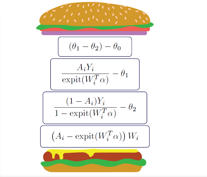
where \(\theta_1\) is the average causal effect, \(\theta_2\) is the mean under the plan where \(A=1\) for everyone, \(\theta_3\) is the mean under the plan where \(A=0\) for everyone, and \(\alpha\) is the parameters for the logistic model used to estimate the propensity scores.
To load the pre-built IPW estimating equations,
from delicatessen.estimating_equations import ee_ipw
The estimating equation is then wrapped inside the wrapper psi function. Notice that the estimating equation has
4 non-optional inputs: the parameter values, the outcomes, the actions, and the covariates to model the propensity
scores with.
def psi(theta):
    return ee_ipw(theta,                 # Parameters
                  y=d['Y'],              # Outcome
                  A=d['A'],              # Action (exposure, treatment, etc.)
                  W=d[['C', 'W']])       # Design matrix for PS model
Note that we add an intercept to the logistic model by adding a column of 1’s via d['C'].
Here, the initial values provided must be 3 + b (where b is the number of columns in W). For binary
outcomes, it will likely be best practice to have the initial values set as [0., 0.5, 0.5, ...]. followed by b
0.’s. For continuous outcomes, all 0. can be used instead. Furthermore, a logistic model for the propensity
scores could be optimized outside of delicatessen and those (pre-washed) regression estimates can be passed as
initial values to speed up optimization.
Now we can call the M-estimator to solve for the values and the variance.
estr = MEstimator(psi, init=[0., 0.5, 0.5, 0., 0.])
estr.estimate(solver='lm')
After successful optimization, we can inspect the estimated values.
estr.theta[0]    # causal mean difference of 1 versus 0
estr.theta[1]    # causal mean under X1
estr.theta[2]    # causal mean under X0
estr.theta[3:]   # logistic regression coefficients
The IPW estimators demonstrates a key advantage of M-estimators. By stacking estimating equations, the sandwich variance estimator correctly incorporates the uncertainty in estimation of the propensity scores into the parameter(s) of interest (e.g., average causal effect). Therefore, we do not have to rely on the nonparametric bootstrap (computationally cumbersome) or the GEE-trick (conservative estimate of the variance for the average causal effect).
G-computation
Second, we use g-computation, which instead models \(Y\) conditional on \(A\) and \(W\). In general, g-computation for the average causal effect can be written as
where \(m_a(W_i; \hat{\beta}) = E[Y_i|A_i=a,W_i; \hat{\beta}]\). In delicatessen, the built-in g-computation
consists of either 2 estimating equations or 4 estimating equations, with both binary and continuous outcomes supported.
The 2 stacked estimating equations are
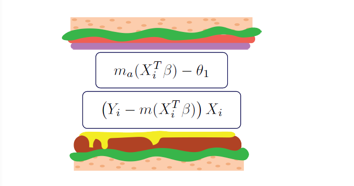
where \(\theta_1\) is the mean under the action \(a\), and \(\beta\) is the parameters for the regression model used to estimate the outcomes. Notice that the g-computation procedure supports generic deterministic plans (e.g., set \(A=1\) for all, set \(A=0\) for all, set \(A=1\) if \(W=1\) otherwise \(A=0\), etc.). These plans are more general than those allowed by either the built-in IPW or built-in AIPW estimating equations.
The 4 stacked estimating equations instead compare the mean difference between two action plans. The estimating equations are
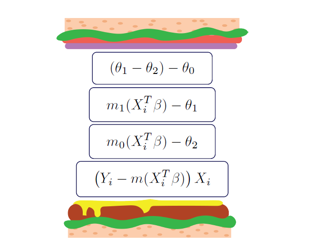
where \(\theta_0\) is the average causal effect, \(\theta_1\) is the mean under the first plan, \(\theta_2\) is the mean under the second, and \(\beta\) is the parameters for the regression model used to predict the outcomes.
To load the pre-built g-computation estimating equations,
from delicatessen.estimating_equations import ee_gformula
The estimating equation is then wrapped inside the wrapper psi function. In the first example, we focus on
estimating the average causal effect. Notice that for ee_gformula some additional data prep is necessary.
Specifically, we need to create a copy of the data set where A is set to the value our plan dictates
(e.g., A=1). Below is code that does this step and creates the wrapper function
# Creating data under the plans
d1 = d.copy()
d1['A'] = 1
d0 = d.copy()
d0['A'] = 0

# Creating interaction terms
d['AxW'] = d['A'] * d['W']
d1['AxW'] = d1['A'] * d1['W']
d0['AxW'] = d0['A'] * d0['W']

def psi(theta):
    return ee_gformula(theta,                        # Parameters
                       y=d['Y'],                     # Outcome
                       X=d[['C', 'A', 'W', 'AxW']],  # Design matrix - observed
                       X=d1[['C', 'A', 'W', 'AxW']], # Design matrix - plan 1
                       X=d0[['C', 'A', 'W', 'AxW']]) # Design matrix - plan 2
Note that we add an intercept to the outcome model by adding a column of 1’s via d['C'].
Here, the initial values provided must be 3+*b* (where b is the number of columns in X). For binary
outcomes, it will likely be best practice to have the initial values set as [0., 0.5, 0.5, ...]. followed by b
0.’s. For continuous outcomes, all 0. can be used instead. Furthermore, a regression model for the outcomes
could be optimized outside of delicatessen and those (pre-washed) regression estimates can be passed as
initial values to speed up optimization.
Now we can call the M-estimator to solve for the values and the variance.
estr = MEstimator(psi, init=[0., 0.5, 0.5, 0., 0., 0., 0.])
estr.estimate(solver='lm')
After successful optimization, we can inspect the estimated values.
estr.theta[0]    # causal mean difference of 1 versus 0
estr.theta[1]    # causal mean under X1
estr.theta[2]    # causal mean under X0
estr.theta[3:]   # regression coefficients
The variance and Wald-type confidence intervals can also be output via
estr.variance
estr.confidence_intervals()
Again, a key advantage of M-Estimation is demonstrated here. By stacking the estimating equations, the sandwich variance estimator correctly incorporates the uncertainty in estimation of the outcome model into the parameter(s) of interest (e.g., average causal effect). Therefore, we do not have to rely on the nonparametric bootstrap.
Augmented inverse probability weighting
Finally, we use the augmented inverse probability weighting (AIPW) esitmator, which incorporates both a model for \(Y\) conditional on \(A\) and \(W\), and a model for \(A\) conditional on \(W\). In other words, the AIPW estimator combines the g-computation and IPW estimators together in a clever way (which has some desireable statistical properties not reviewed here). The AIPW estimator for the average causal effect can be written as
where \(m_a(W_i; \hat{\beta}) = E[Y_i|A_i=a,W_i; \hat{\beta}]\), and
\(\pi_i = Pr(A_i = 1 | W_i; \hat{\alpha})\). In delicatessen, the built-in AIPW estimator consists of 5
estimating equations, with both binary and continuous outcomes supported. Similar to IPW (and unlike g-computation),
the built-in AIPW estimator only supports the average causal effect as the parameter of interest.
The stacked estimating equations are
where \(\theta_0\) is the average causal effect, \(\theta_1\) is the mean under the first plan, \(\theta_2\) is the mean under the second, \(\alpha\) is the parameters for the propensity score logistic model, and \(\beta\) is the parameters for the regression model used to predict the outcomes. For binary outcomes, the final estimating equation is replaced with the logistic model analog.
To load the pre-built AIPW estimating equations,
from delicatessen.estimating_equations import ee_aipw
The estimating equation is then wrapped inside the wrapper psi function. Like ee_gformula, ee_aipw requires
some additional data prep. Specifically, we need to create a copy of the data set where \(A=1\) for everyone and another
copy where \(A=0\) for everyone. Below is code that does this step and creates the wrapper function
# Creating data under the plans
d1 = d.copy()
d1['A'] = 1
d0 = d.copy()
d0['A'] = 0

# Creating interaction terms
d['AxW'] = d['A'] * d['W']
d1['AxW'] = d1['A'] * d1['W']
d0['AxW'] = d0['A'] * d0['W']

def psi(theta):
    return ee_gformula(theta,                        # Parameters
                       y=d['Y'],                     # Outcome
                       A=d['A'],                     # Action
                       W=d[['C', 'W']],              # Design matrix - PS
                       X=d[['C', 'A', 'W', 'AxW']],  # Design matrix - observed
                       X=d1[['C', 'A', 'W', 'AxW']], # Design matrix - plan A=1
                       X=d0[['C', 'A', 'W', 'AxW']]) # Design matrix - plan A=0
Note that we add an intercept to the outcome model by adding a column of 1’s via d['C'].
Here, the initial values provided must be 3 + b + c (where b is the number of columns in W and c is the number
of columns in X). For binary outcomes, it will likely be best practice to have the initial values set as
[0., 0.5, 0.5, ...]. followed by b 0.’s. For continuous outcomes, all 0. can be used instead. Furthermore,
a regression models could be optimized outside of delicatessen and those (pre-washed) regression estimates can be
passed as initial values to speed up optimization.
Now we can call the M-estimator to solve for the values and the variance.
estr = MEstimator(psi, init=[0., 0.5, 0.5,
                             0., 0.,
                             0., 0., 0., 0.])
estr.estimate(solver='lm')
After successful optimization, we can inspect the estimated values.
estr.theta[0]     # causal mean difference of 1 versus 0
estr.theta[1]     # causal mean under A=1
estr.theta[2]     # causal mean under A=0
estr.theta[3:5]   # propensity score regression coefficients
estr.theta[5:]    # outcome regression coefficients
The variance and Wald-type confidence intervals can also be output via
estr.variance
estr.confidence_intervals()
Additional Examples
For additional examples, we have replicated chapters 12-14 of the textbook “Causal Inference: What If” by Hernan and Robins (2023). These additional examples are provided here.
References and Further Readings
Boos DD, & Stefanski LA. (2013). M-estimation (estimating equations). In Essential Statistical Inference (pp. 297-337). Springer, New York, NY.
Cole SR, & Hernán MA. (2008). Constructing inverse probability weights for marginal structural models. American Journal of Epidemiology, 168(6), 656-664.
Funk MJ, Westreich D, Wiesen C, Stürmer T, Brookhart MA, & Davidian M. (2011). Doubly robust estimation of causal effects. American Journal of Epidemiology, 173(7), 761-767.
Hernán MA, & Robins JM. (2006). Estimating causal effects from epidemiological data. Journal of Epidemiology & Community Health, 60(7), 578-586.
Huber PJ. (1992). Robust estimation of a location parameter. In Breakthroughs in statistics (pp. 492-518). Springer, New York, NY.
Inderjit, Streibig JC & Olofsdotter M. (2002). Joint action of phenolic acid mixtures and its significance in allelopathy research. Physiol Plant 114, 422–428.
Snowden JM, Rose S, & Mortimer KM. (2011). Implementation of G-computation on a simulated data set: demonstration of a causal inference technique. American Journal of Epidemiology, 173(7), 731-738.